BATSE PHAII Data (gdt.missions.cgro.batse.phaii)

The primary science data produced by BATSE can be summarized as a time history of spectra, which is mostly provided as temporally pre-binned data, and some small amount of temporally unbinned (TTE) data around on-board triggers. These data types are produced as “snippets” for every single trigger and some are also provided continuously. There are generally two different types of files that contain BATSE PHAII data: files that contain PHAII data for a single detector and files that contain PHAII data for multiple detectors. Both of these types can be read with BatsePhaii.

Reading Multi-Detector PHAII Files

Here is an example of reading a daily continuous file containing multiple detectors:

>>> from gdt.core import data_path
>>> from gdt.missions.cgro.batse.phaii import BatsePhaii
>>> filepath = data_path / 'cgro-batse' / 'cont_08362.fits.gz'
>>> phaii_multi = BatsePhaii.open(filepath)
>>> phaii_multi
<BatsePhaiiMulti: 8 detectors>

As you can see, reading this file returns a BatsePhaiiMulti object, which contains the PHAII data for multiple detectors. In this example, the file contains data from all 8 LADs, but this isn’t always the case. We can retrieve a list of detector numbers that are in the file:

>>> phaii_multi.detectors
[0, 1, 2, 3, 4, 5, 6, 7]

If we want to retrieve a particular detector from the file, we can do that with the following:

>>> # retrieve the PHAII data for LAD 3
>>> phaii3 = phaii_multi.get_detector(3)
>>> phaii3
<BatsePhaiiCont:
 time range (8362.557340507052, 8362.997613099642);
 energy range (21.800001, 3999.9998)>

As you can see, a BatsePhaiiCont object is returned, which is simply a type of BatsePhaii object. Since these files are in the FITS format, the header information is populated when retrieving a detector:

>>> phaii3.headers.keys()
['PRIMARY', 'BATSE_E_CALIB', 'BATSE_CNTS']

>>> phaii3.headers['PRIMARY']
TELESCOP= 'COMPTON GRO'
INSTRUME= 'BATSE   '
ORIGIN  = 'MSFC    '           / Tape writing institution
FILETYPE= 'BATSE_CONT'
OBSERVER= 'G. J. Fishman'      / Principal investigator (256) 544-7691
TJD     =                 8362 / TJD at start of data
STRT-DAY=             1991.106 / YYYY.DDD at start of data
STRT-TIM=                  1.0 / seconds of day at start of data
END-DAY =             1991.106 / YYYY.DDD at end of data
END-TIM =              86398.0 / seconds of day at end of data
N_E_CHAN=                   16 / number of energy channels
TIME_RES=                2.048 / Time resolution of data (second)
EQUINOX =               2000.0 / J2000 coordinates
SC-Z-RA =              108.149 / Z axis RA in degrees
SC-Z-DEC=               -6.583 / Z axis Dec in degrees
SC-X-RA =                19.08 / X axis RA in degrees
SC-X-DEC=                8.022 / X axis Dec in degrees
SC-Z-LII=             -138.797 / Z axis Galactic coordinate LII in degr
SC-Z-BII=                1.675 / Z axis Galactic coordinate BII in degr
SC-X-LII=              133.537 / X axis Galactic coordinate LII in degr
SC-X-BII=              -54.337 / X axis Galactic coordinate BII in degr
QMASKDAT= 'CONFITS1'           / mask used for data filtering
QMASKHKG= 'OHEDIT2 '           / mask used for housekeeping data filtering
FILE-ID = 'CONT_08362.FITS'    / Name of FITS file
FILE-VER= 'V1.00   '           / Version of FITS file format
FILENAME= '[.DDS08362]CONTINUOUS_DATA.DAT DDS08362' / Original File
CDATE   = '2-JUL-2002 15:41:30.59' / Date FITS file created
MNEMONIC= 'CONT_DISCLA_FITS 4.10' / Program creating this file
PRIMTYPE= 'NONE    '           / No primary array

There is easy access for certain important properties of the data:

>>> # the good time intervals for the data
>>> phaii3.gti
<Gti: 1 intervals; range (8362.557340507052, 8362.997613099642)>

>>> # the time range
>>> phaii3.time_range
(8362.557340507052, 8362.997613099642)

>>> # the energy range
>>> phaii3.energy_range
(21.800001, 3999.9998)

>>> # number of energy channels
>>> phaii3.num_chans
16

Note

The time values are based on the CGRO mission epoch and format, which is Truncated Julian Date and details can be found here `cgro-time`_.

Working with BATSE PHAII objects

We can retrieve the time history spectra data contained within the file, which is a TimeEnergyBins class (see 2D Binned Data for more details).

>>> phaii3.data
<BatseTimeEnergyBins: 4485 time bins;
 time range (8362.557340507052, 8362.997613099642);
 7 time segments;
 16 energy bins;
 energy range (21.800001, 3999.9998);
 1 energy segments>

Through the Phaii base class, there are a lot of high level functions available to us, such as slicing the data in time or energy:

>>> time_sliced_phaii3 = phaii3.slice_time((8362.6, 8362.7))
>>> time_sliced_phaii3
<BatsePhaiiCont:
 time range (8362.557814581125, 8362.700013099642);
 energy range (21.800001, 3999.9998)>

>>> energy_sliced_phaii3 = phaii3.slice_energy((50.0, 500.0))
>>> energy_sliced_phaii3
<BatsePhaiiCont:
 time range (8362.557340507052, 8362.997613099642);
 energy range (21.800001, 601.1419)>

As mentioned, this data is 2-dimensional, so what do we do if we want a lightcurve covering a particular energy range? We integrate (sum) over energy, and we can easily do this:

>>> lightcurve = phaii3.to_lightcurve(energy_range=(50.0, 500.0))
>>> lightcurve
<BatseTimeBins: 4485 bins;
 range (8362.557340507052, 8362.997613099642);
 7 contiguous segments>

Similarly, we can integrate over time to produce a count spectrum:

>>> spectrum = phaii3.to_spectrum(time_range=(8362.6, 8362.7))
>>> spectrum
<EnergyBins: 16 bins;
 range (21.800001, 3999.9998);
 1 contiguous segments>

The resulting objects are TimeBins and EnergyBins, respectively, and see 1D Binned Data for more details on how to use them.

Of course, once we have produced a lightcurve or spectrum data object, often we want to plot it. For that, we use the Lightcurve and Spectrum plotting classes:

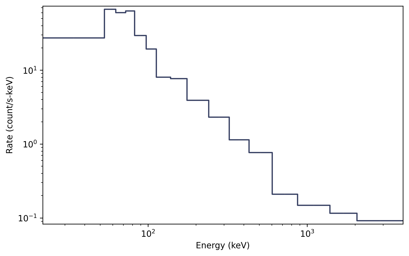
>>> import matplotlib.pyplot as plt
>>> from gdt.core.plot.lightcurve import Lightcurve
>>> lcplot = Lightcurve(data=lightcurve)
>>> lcplot.errorbars.hide()
>>> plt.show()

This plot shows the lightcurve over a full day of observations. The dropouts in the lightcurve is when the detector is turned off, most likely as CGRO was passing through the South Atlantic Anomaly.

We can zoom in to a particular region of the plot and uncover a GRB-like signal:

>>> lcplot.xlim = (8362.84, 8362.85)
>>> lcplot.ylim = (4000, 6000)

Similarly, we can plot the count spectrum:

>>> from gdt.core.plot.spectrum import Spectrum
>>> specplot = Spectrum(data=spectrum)
>>> plt.show()

See Plotting Lightcurves and Plotting Count Spectra for more on how to modify these plots.

Reading BATSE trigger PHAII files

Similarly, we can read triggered BATSE PHAII, which mostly keep to a single detector per file. For example:

>>> filepath = data_path / 'cgro-batse' / 'cont_bfits_3_105.fits.gz'
>>> phaii_trig = BatsePhaii.open(filepath)
>>> phaii_trig
<BatsePhaiiTrigger: cont_bfits_3_105.fits.gz;
 trigger time: 8367.384765694444;
 time range (-120.83200073242188, 38.9119987487793);
 energy range (13.140961, 100000.0)>

Notice that the object is a BatsePhaiiTrigger, which is a special type of BatsePhaii object. All of the same attributes and functions we looked at for the multi-detector files apply here. For example, we can plot the full-band lightcurve:

>>> lc = phaii_trig.to_lightcurve()
>>> lcplot = Lightcurve(data=lc)
>>> plt.show()

Notice that the times here are relative to the trigger time:

>>> phaii_trig.trigtime
8367.384765694444

There are many different types of BATSE data that can be accessed and analyzed using the GDT. For a listing of these data types and visual examples, see the BATSE Data File Gallery.

For more details about working with PHAII data, see PHAII Files.

Reference/API

gdt.missions.cgro.batse.phaii Module

Classes

BatsePhaii()	Class representing BATSE PHAII data.
BatsePhaiiMulti()	BATSE data containing PHAII from multiple detectors.
BatsePhaiiCont()	The continuous CONT data.
BatsePhaiiDiscla()	The continuous LAD discriminator data.
BatsePhaiiTrigger()	Class representing trigger BATSE PHAII data.
BatseEnergyCalib()	BATSE Energy Calibration data, which is stored in PHAII and event list files.

Class Inheritance Diagram